Mathematics

The Basic Fitting Interface

MATLAB supports curve fitting through the Basic Fitting interface. Using this interface, you can quickly perform many curve fitting tasks within the same easy-to-use environment. The interface is designed so that you can

• Fit data using a spline interpolant, a shape-preserving interpolant, or a polynomial up to degree 10
• Plot multiple fits simultaneously for a given data set
• Plot the fit residuals
• Examine the numerical results of a fit
• Evaluate (interpolate or extrapolate) a fit
• Annotate the plot with the numerical fit results and the norm of residuals
• Save the fit and evaluated results to the MATLAB workspace

Depending on your specific curve fitting application, you can use the Basic Fitting interface, the command line functionality, or both.

You can use the Basic Fitting interface only with 2-D data. However, if you plot multiple data sets as a subplot, and at least one data set is 2-D, then the interface is enabled.

Improving Fitting Efficiency

MATLAB does not sort your data before fitting it with the Basic Fitting interface, although it did so in prior releases. This change in behavior was made to improve handling of residual plots. However, as sorted data is faster to fit and plot, you can improve performance of the Basic Fitting interface with large data sets by presorting your data so that the x values are in ascending order. If your original data consists of the vectors x and y, you can create sorted vectors x_sorted and y_sorted as follows:

• [x_sorted, i] = sort(x);
  y_sorted = y(i);
  

Overview of the Basic Fitting Interface

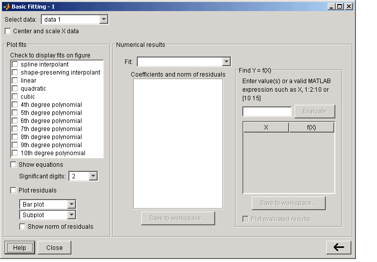
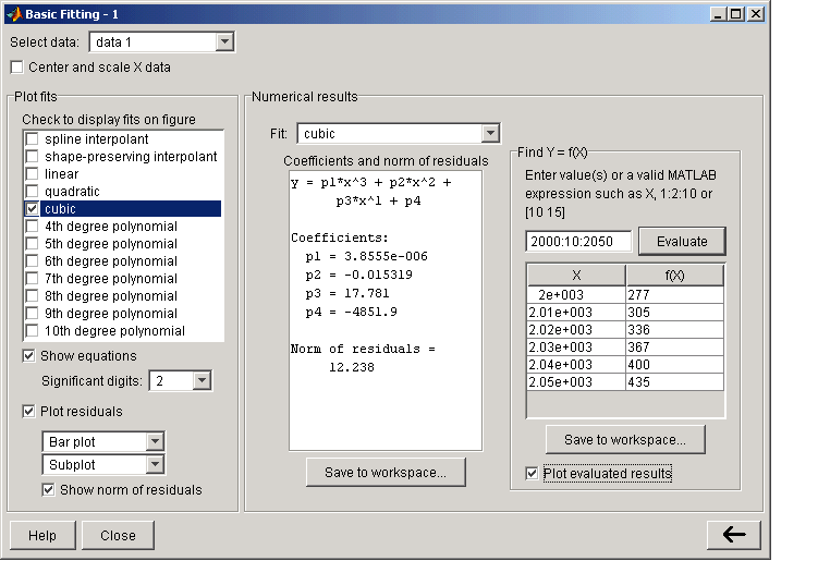
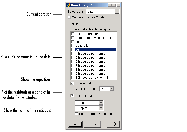
The full Basic Fitting interface is shown below. To reproduce this state, follow these three steps:

1. Plot some data.
2. Select Basic Fitting from the Tools menu.
3. Click the button twice.

   

Select data - This parameter list is populated with the names of all the data sets you display in the figure window associated with the Basic Fitting interface.

Use this list to select the current data set -- the data set that you want to fit. You can fit only one data set at a time. However, you can perform multiple fits for the current data set. Use the Plot Editor to change the name of a data set.

Center and scale X data - If checked, the data is centered at zero mean and scaled to unit standard deviation. You may need to center and scale your data to improve the accuracy of the subsequent numerical computations. MATLAB displays a warning is displayed if a fit produces results that might be inaccurate.

Plot fits - This panel enables you to visually explore one or more fits to the current data set:

• Check to display fits on figure - Select the fits you want to display for the current data set. There are two types of fits to choose from: interpolants and polynomials. The spline interpolant uses the spline function, while the shape-preserving interpolant uses the pchip function. Refer to the pchip online help for a comparison of these two functions. The polynomial fits use the polyfit function. You can choose as many fits for a given data set as you want.

• If your data set has N points, then you should use polynomials with, at most, N coefficients. If your fit uses polynomials with more than N coefficients, the interface automatically sets a sufficient number of coefficients to 0 during the calculation so that the system is not underdetermined.

• Show equations - If checked, the fit equation is displayed on the plot.
• Significant digits - Select the significant digits associated with the equation display.
• Plot residuals - If checked, the fit residuals are displayed. The fit residuals are defined as the difference between the ordinate data point and the resulting fit for each abscissa data point. You can display the residuals as a bar plot, as a scatter plot, or as a line plot in the same figure window as the data or in a separate figure window. If you use subplots to plot multiple data sets, then residuals can be plotted only in a separate figure window.
• Show norm of residuals - If checked, the norm of residuals are displayed. The norm of residuals is a measure of the goodness of fit, where a smaller value indicates a better fit than a larger value. It is calculated using the norm function, norm(V,2), where V is the vector of residuals.

Numerical results - This panel allows you to explore the numerical results of a single fit to the current data set without plotting the fit:

• Fit - Select the equation to fit to the current data set. The fit results are displayed in the list box below the menu. Note that selecting an equation in this menu does not affect the state of the Plot fits panel. Therefore, if you want to display the fit in the data plot, you may need to select the associated check box in Plot fits.
• Coefficients and norm of residuals - Display the numerical results for the equation selected in Fit. Note that when you first open the Numerical Results panel, the results of the last fit you selected in Plot fits are displayed.
• Save to workspace - Launch a dialog box that allows you to save the fit results to workspace variables.
• Find Y = f(X) - Interpolate or extrapolate the current fit.
• Enter value(s) - Enter a MATLAB expression to evaluate for the current fit. The expression is evaluated after you press the Evaluate button, and the results are displayed in the associated table. The current fit is displayed in the Fit menu.
• Save to workspace - Launch a dialog box that allows you to save the evaluated results to workspace variables.
• Plot results - If checked, the evaluated results are displayed on the data plot.

Example: Using the Basic Fitting Interface

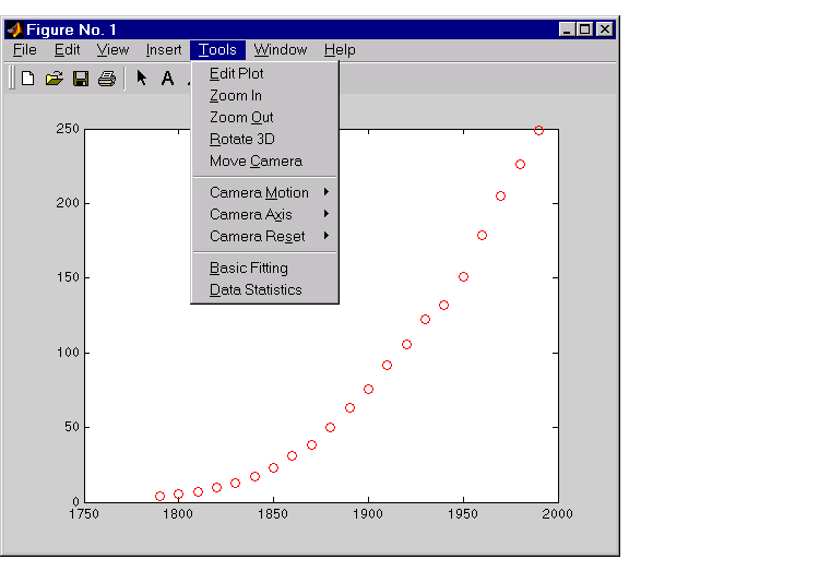
This example illustrates the features of the Basic Fitting interface by fitting a cubic polynomial to the census data. You may want to repeat this example using different equations and compare results. To launch the interface:

1. Plot some data.

• plot(cdate,pop,'ro')
  

2. Select Basic Fitting from the Tools menu in the figure.

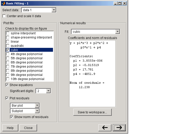
Configure the Basic Fitting interface to:

• Fit a cubic polynomial to the data.
• Display the equation in the data plot.
• Plot the fit residuals as a bar plot, and display the residuals as a subplot of the data figure window.
• Display the norm of the residuals.

This configuration is shown below.

The Plot fits panel enables you to visually explore multiple fits to the current data set. For comparison, try fitting additional equations to the census data by selecting the appropriate check boxes. If an equation produces results that might be numerically inaccurate, MATLAB displays a warning. In this case, you should select the Center and scale X data check box to improve the numerical accuracy.

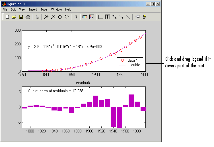
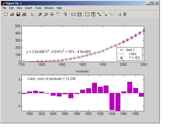
The resulting fit and the residuals are shown in the following plot.

The plot legend indicates the name of the data set and the equation. If the legend covers part of the plot, you can click and drag it to another location. The legend is automatically updated as you add or remove data sets or fits. Additionally, fits are displayed using a default set of line styles and colors. You can change any of the default plot settings using the Plot Editor. However, any changes you make are undone if you subsequently perform another fit. To retain changes, you should wait until after you have finished fitting your data.

Note    If you change the name of a data set in the legend, then the name is automatically changed in the Select data menu.

By selecting the button, you can examine the fit coefficients and the norm of the residuals.

The Fit menu enables you to explore numerical fit results for the current data set without plotting the fit. For comparison, you can display the numerical results for other fits by selecting the desired equation. Note that if you want to display a fit in the data plot, you have to select the associated check box in Plot fits.

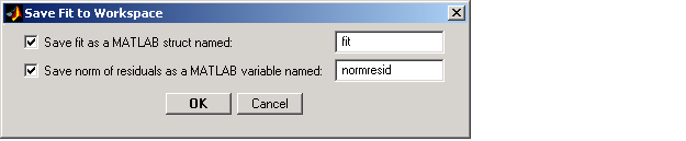
You can save the fit results to the MATLAB workspace by selecting the Save to workspace button.

The fit structure is

• fit1
  fit1 = 
       type: 'polynomial degree 3'
      coeff: [3.8555e-006 -0.0153 17.7815 -4.8519e+003]
  

You may want to use this structure for subsequent display or analysis. For example, you can use the saved coefficients and the polyval function to evaluate the cubic polynomial at the command line.

By selecting the button again, you can specify a vector of x-values at which to evaluate the current fit. Enter the vector in the field next to the Evaluate button, and then click Evaluate. For example, if you enter the vector 2000:10:2050, the population for the years 2000 to 2050 is evaluated in increments of 10. The x-values and the corresponding values for f(x), evaluated from the fit, are displayed in the pane below Evaluate, as shown in the following figure.

Select the Plot evaluated results check box to display the evaluated points along with the current data set in the data plot, as shown in the following figure.

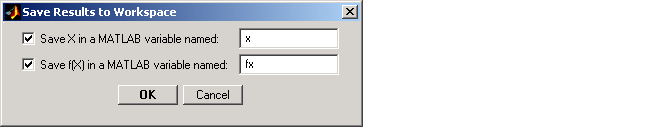
You can save the evaluated data to the MATLAB workspace by selecting the Save to workspace button.

Error Bounds

Difference Equations and Filtering

© 1994-2005 The MathWorks, Inc.