Design (newhop) :: Recurrent Networks (Neural Network Toolbox)

Neural Network Toolbox

Design (newhop)

Li et al. [LiMi89] have studied a system that has the basic structure of the Hopfield network but is, in Li's own words, "easier to analyze, synthesize, and implement than the Hopfield model." The authors are enthusiastic about the reference article, as it has many excellent points and is one of the most readable in the field. However, the design is mathematically complex, and even a short justification of it would burden this guide. Thus, we present the Li design method, with thanks to Li et al., as a recipe that is found in the function newhop.

Given a set of target equilibrium points represented as a matrix T of vectors, newhop returns weights and biases for a recursive network. The network is guaranteed to have stable equilibrium points at the target vectors, but it could contain other spurious equilibrium points as well. The number of these undesired points is made as small as possible by the design method.

Once the network has been designed, it can be tested with one or more input vectors. Hopefully those input vectors close to target equilibrium points will find their targets. As suggested by the network figure, an array of input vectors may be presented at one time or in a batch. The network proceeds to give output vectors that are fed back as inputs. These output vectors can be can be compared to the target vectors to see how the solution is proceeding.

The ability to run batches of trial input vectors quickly allows you to check the design in a relatively short time. First you might check to see that the target equilibrium point vectors are indeed contained in the network. Then you could try other input vectors to determine the domains of attraction of the target equilibrium points and the locations of spurious equilibrium points if they are present.

Consider the following design example. Suppose that we want to design a network with two stable points in a three-dimensional space.

T = [-1 -1 1; 1 -1 1]'
T =
    -1     1
    -1    -1
     1     1

We can execute the design with

```
net = newhop(T);
```

Next we can check to make sure that the designed network is at these two points. We can do this as follows. (Since Hopfield networks have no inputs, the second argument to sim below is Q = 2 when using matrix notation).

Ai = T;
[Y,Pf,Af] = sim(net,2,[],Ai);
Y

This gives us

Thus, the network has indeed been designed to be stable at its design points. Next we can try another input condition that is not a design point, such as:

```
Ai = {[-0.9; -0.8; 0.7]}
```

This point is reasonably close to the first design point, so one might anticipate that the network would converge to that first point. To see if this happens, we run the following code. Note, incidentally, that we specified the original point in cell array form. This allows us to run the network for more than one step.

```
[Y,Pf,Af] = sim(net,{1 5},{},Ai);
Y{1}
```

We get

```
Y =
    -1
    -1
     1
```

Thus, an original condition close to a design point did converge to that point.

This is, of course, our hope for all such inputs. Unfortunately, even the best known Hopfield designs occasionally include undesired spurious stable points that attract the solution.

Example

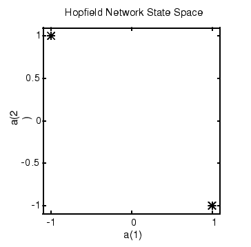
Consider a Hopfield network with just two neurons. Each neuron has a bias and weights to accommodate two-element input vectors weighted. We define the target equilibrium points to be stored in the network as the two columns of the matrix T.

T = [1 -1; -1 1]'
T =
     1    -1
    -1     1

Here is a plot of the Hopfield state space with the two stable points labeled with `*' markers.

These target stable points are given to newhop to obtain weights and biases of a Hopfield network.

```
net = newhop(T);
```

The design returns a set of weights and a bias for each neuron. The results are obtained from

```
W= net.LW{1,1}
```

which gives

W =
    0.6925   -0.4694
   -0.4694    0.6925

and from

```
b = net.b{1,1}
```

which gives

```
b =
   1.0e-16 *
    0.6900
    0.6900
```

Next the design is tested with the target vectors T to see if they are stored in the network. The targets are used as inputs for the simulation function sim.

Ai = T;
[Y,Pf,Af] = sim(net,2,[],Ai);
Y =
     1    -1
    -1     1

As hoped, the new network outputs are the target vectors. The solution stays at its initial conditions after a single update and, therefore, will stay there for any number of updates.

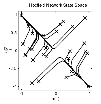
Now you might wonder how the network performs with various random input vectors. Here is a plot showing the paths that the network took through its state space, to arrive at a target point.

This plot shows the trajectories of the solution for various starting points. You can try the demonstration demohop1 to see more of this kind of network behavior.

Hopfield networks can be designed for an arbitrary number of dimensions. You can try demohop3 to see a three-dimensional design.

Unfortunately, Hopfield networks could have both unstable equilibrium points and spurious stable points. You can try demonstration programs demohop2 and demohop4 to investigate these issues.

Architecture Summary