Wavelet Toolbox

One-Stage Filtering: Approximations and Details

For many signals, the low-frequency content is the most important part. It is what gives the signal its identity. The high-frequency content, on the other hand, imparts flavor or nuance. Consider the human voice. If you remove the high-frequency components, the voice sounds different, but you can still tell what's being said. However, if you remove enough of the low-frequency components, you hear gibberish.

In wavelet analysis, we often speak of approximations and details. The approximations are the high-scale, low-frequency components of the signal. The details are the low-scale, high-frequency components.

The filtering process, at its most basic level, looks like this:

The original signal, S, passes through two complementary filters and emerges as two signals.

Unfortunately, if we actually perform this operation on a real digital signal, we wind up with twice as much data as we started with. Suppose, for instance, that the original signal S consists of 1000 samples of data. Then the resulting signals will each have 1000 samples, for a total of 2000.

These signals A and D are interesting, but we get 2000 values instead of the 1000 we had. There exists a more subtle way to perform the decomposition using wavelets. By looking carefully at the computation, we may keep only one point out of two in each of the two 2000-length samples to get the complete information. This is the notion of downsampling. We produce two sequences called cA and cD.

The process on the right, which includes downsampling, produces DWT coefficients.

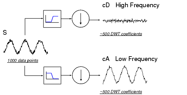
To gain a better appreciation of this process, let's perform a one-stage discrete wavelet transform of a signal. Our signal will be a pure sinusoid with high-frequency noise added to it.

Here is our schematic diagram with real signals inserted into it:

The MATLAB code needed to generate s, cD, and cA is

• s = sin(20.*linspace(0,pi,1000)) + 0.5.*rand(1,1000);
  [cA,cD] = dwt(s,'db2');
  

where db2 is the name of the wavelet we want to use for the analysis.

Notice that the detail coefficients cD are small and consist mainly of a high-frequency noise, while the approximation coefficients cA contain much less noise than does the original signal.

• [length(cA) length(cD)]
  
  ans =
     501  501
  

You may observe that the actual lengths of the detail and approximation coefficient vectors are slightly more than half the length of the original signal. This has to do with the filtering process, which is implemented by convolving the signal with a filter. The convolution "smears" the signal, introducing several extra samples into the result.

The Discrete Wavelet Transform

Multiple-Level Decomposition

© 1994-2005 The MathWorks, Inc.