Wavelet Toolbox

One-Dimensional Estimation Using the GUI for Equally Spaced Observations (Fixed Design)

1. Start the Regression Estimation 1-D Tool.

1. From the MATLAB prompt, type

   • wavemenu
     

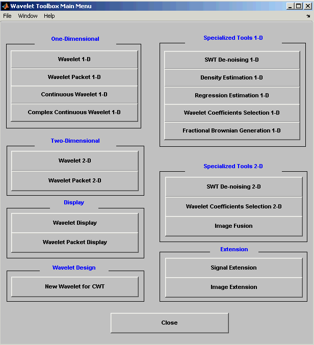
   The Wavelet Toolbox Main Menu appears.
   
   

   Click the Regression Estimation 1-D menu item. The discrete wavelet analysis tool for one-dimensional regression estimation appears.

   

2. Load data.

1. From the File menu, choose the Load Data for Fixed Design Regression option.

   

   When the Load data for Fixed Design Regression dialog box appears, select the demo MAT-file noisbloc.mat, which should reside in the MATLAB directory toolbox/wavelet/wavedemo.

   Click the OK button. The noisy blocks data is loaded into the Regression Estimation 1-D - Fixed Design tool.

   

   The loaded data denoted (X,Y) and the processed data obtained after a binning, are displayed.

3. Choose the processed data.

1. The default value for the number of bins is 256 for this example. Enter 64 in the Nb bins (number of bins) edit box, or use the slider to adjust the value. The new binned data to be processed appears.

   

   The binned data appears to be very smoothed. Select 1000 from the Nb bins edit and press Enter or use the slider. The new data to be processed appears.

   

   The binned data appears to be very close to the initial data, since noisbloc is of length 1024.

4. Perform a Wavelet Decomposition of the processed data.

1. Select the haar wavelet from the Wavelet menu and select 5 from the Level menu, and then click the Decompose button. After a pause for computation, the tool displays the detail coefficients of the decomposition.

   

5. Perform a regression estimation.

1. While a number of options are available for fine-tuning the estimation algorithm, we'll accept the defaults of fixed form soft thresholding and unscaled white noise. The sliders located to the right of the window control the level dependent thresholds, indicated by yellow dotted lines running horizontally through the graphs on the left part of the window.

   Continue by clicking the Estimate button.

   

   You can see that the process removed the noise and that the blocks are well reconstructed. The regression estimate (in yellow) is the sum of the signals located below it: the approximation a5 and the reconstructed details after coefficient thresholding.

   You can experiment with the various predefined thresholding strategies by selecting the appropriate options from the menu located on the right part of the window or directly by dragging the yellow horizontal lines with the left mouse button.

   Let us now illustrate the regression estimation using the graphical interface for randomly or irregularly spaced observations, focusing on the differences from the previous situation.

One-Dimensional Wavelet Regression Estimation

One-Dimensional Estimation Using the GUI for Randomly Spaced Observations (Stochastic Design)

© 1994-2005 The MathWorks, Inc.