wfbmesti (Wavelet Toolbox)

Parameter estimation of fractional Brownian motion

Syntax

```
HEST = wfbmesti(X)
```

Description

HEST = wfbmesti(X) returns a row vector HEST which contains three estimates of the fractal index H of the signal X supposed to come from a fractional Brownian motion of parameter H.

The two first estimates are based on second order discrete derivative, the second one is wavelet-based.

The third estimate is based on the linear regression in loglog plot, of the variance of detail versus level.

A fractional Brownian motion (fBm) is a continuous-time Gaussian process depending on the so-called Hurst parameter 0 < H < 1. It generalizes the ordinary Brownian motion corresponding to H = 0.5 and whose derivative is the white noise. The fBm is self-similar in distribution and the variance of the increments is given by

```
Var(fBm(t)-fBm(s)) = v |t-s|^2H
```

where v is a positive constant.

This special form of the variance of the increments suggests various ways to estimate the parameter H. One can find in Bardet et al. a survey of such methods. The wfbmesti M-file provides three different estimates. The first one, due to Istas and Lang, is based on the discrete second-order derivative. The second one is a wavelet-based adaptation and has similar properties. The third one, proposed by Flandrin, estimates H using the slope of the loglog plot of the detail variance versus the level. A more recent extension can be found in Abry et al.

Examples

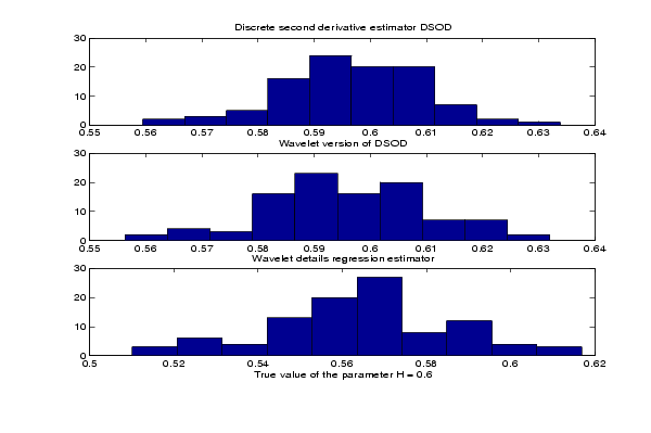
This example shows a statistical comparison of the three estimators by a short Monte-Carlo study.

% Initialize the randn generator
randn('state',1)

% Set parameter H to 0.6 and sample length
H = 0.6; lg = 10000;
% Generate 100 wavelet-based fBm realizations for H = 0.6
% and compute the three estimates for each of them
n = 100; Hest = zeros(n,3);
for i = 1:n
    fBm06 = wfbm(H,lg);
    Hest(i,:) = wfbmesti(fBm06);
end

% Compare empirical distributions
subplot(311), hist(Hest(:,1)); 
title('Discrete second derivative estimator DSOD')
subplot(312), hist(Hest(:,2)); 
title('Wavelet version of DSOD') 
subplot(313), hist(Hest(:,3)); 
title('Wavelet details regression estimator')
xlabel('True value of the parameter H = 0.6')

For these experimental conditions, the two first methods give similar results with smaller dispersion than the third one. The third one is clearly slightly biased and has greater dispersion.

These experimental results depend on H and on the various experimental conditions, for a complete study, see Bardet et al.

See Also

wfbm

References

Abry, P.; P. Flandrin, M.S. Taqqu, D. Veitch (2003), "Self-similarity and long-range dependence through the wavelet lens," Theory and applications of long-range dependence, Birkhäuser, pp. 527-556.

Bardet, J.-M.; G. Lang, G. Oppenheim, A. Philippe, S. Stoev, M.S. Taqqu (2003), "Semi-parametric estimation of the long-range dependence parameter: a survey," Theory and applications of long-range dependence, Birkhäuser, pp. 557-577.

Flandrin, P. (1992), "Wavelet analysis and synthesis of fractional Brownian motion," IEEE Trans. on Inf. Th., 38, pp. 910-917.

Istas, J.; G. Lang (1994), "Quadratic variations and estimation of the local Hölder index of a Gaussian process," Ann. Inst. Poincaré, 33, pp. 407-436.

wfbm wfilters