

| MATLAB Release Notes | |
Mathematics Features
MATLAB 7.0 adds the following mathematics features and enhancements:
New Nondouble Mathematics Features
MATLAB Version 7.0 now supports many arithmetic operations and mathematical functions on the following nondouble MATLAB data types:
Most of the built-in MATLAB functions that perform mathematical operations now support inputs of type single. In addition, the arithmetic operators and the functions sum, diff, colon, and some elementary functions now support integer data types.
This section covers the following topics:
Nondouble Arithmetic
This section describes how MATLAB performs arithmetic on nondouble data types.
Single Arithmetic. You can now combine numbers of type single with numbers of type double or single. MATLAB performs arithmetic as if both inputs had type single and returns a result of type single. For more information, see Single-Precision Mathematics in the online MATLAB documentation.
Integer Arithmetic. You can now combine numbers of an integer data type with numbers of the same integer data type or type scalar double. MATLAB performs arithmetic as if both inputs had type double and then converts the result to the same integer data type.
MATLAB computes operations on arrays of integer data type using saturating integer arithmetic. Saturating means that if the result is greater than the upper bound of the integer data type, MATLAB returns the upper bound. Similarly, if the result is less than the lower bound of the data type, MATLAB returns the lower bound. For more information, see Integer Mathematics in the online MATLAB documentation.
New Class and Data Inputs for eps
You can now call the function eps with the syntax
If x has type double, eps(x) returns the distance from x to the next largest double-precision floating point number. This is a measure of the accuracy of x as a double-precision number. eps(1) returns the same value as eps with no input argument.
You can now replace expressions of the form
If x has type single, eps(x) returns the distance from x to the next largest single-precision floating point number. This is a measure of the accuracy of x as a single-precision number.
returns the same value as eps(single(1)). The value of eps('single') is the same as single(2^-23). The command eps('double') returns the same result as eps.
See eps in Double and Single-Precision Arithmetic in the online MATLAB documentation for more information.
New Class Inputs for realmax and realmin
You can now call the function realmax with the syntax
which returns the largest single-precision number. Similarly,
returns the smallest single-precision number.
The commands realmax('double') and realmin('double') return the same results as realmax and realmin, respectively. See Largest and Smallest Numbers in the online MATLAB documentation for more information.
New Functions intmax and intmin
Two new functions, intmax and intmin, return the largest and smallest numbers, respectively, for integer data types. For example,
returns the largest number of type int8. See Largest and Smallest Values for Integer Data Types in the online MATLAB documentation for more information.
New Warnings for Integer Arithmetic
This section describes four new warning messages for integer arithmetic in Version 7.0. While these warnings are turned off by default, you can turn them on as a diagnostic tool or to warn of behavior in integer arithmetic that might not be expected.
To turn all four warning messages on at once, enter
Integer Conversion of Noninteger Values. MATLAB can now return a warning when it rounds up a number in converting to an integer data type. For example,
int8(2.7)
Warning: Conversion rounded non-integer floating point value to
nearest int8 value.

ans =

    3
Integer Conversion of NaN. When MATLAB converts NaN (Not-a-Number) to an integer data type, the result is 0. MATLAB can now return a warning when this occurs. For example,
Integer Conversion Overflow. MATLAB can now return a warning when you convert a number to an integer data type and the number is outside the range of the data type. For example,
Integer Arithmetic Overflow. MATLAB can now return a warning when the result of an operation on integer data types is either NaN or outside the range of that data type. For example,
To turn all of these warnings off at once, enter
New Class Inputs for ones, zeros, and eye
You can now call ones or zeros with an input argument specifying the data type of the output. For example,
returns an m-by-n-by-p-by ... array of type single containing all ones. zeros uses the same syntax.
You can now call eye with this input argument for two-dimensional arrays. For example,
returns an m-by-m identity matrix of type single. The command
returns an m-by-n array of type int8.
New Class and Size Inputs for Inf and NaN
The functions Inf and NaN now accept inputs that enable you to create Infs or NaNs of specified sizes and floating-point data types. As examples,
Inf('single') or NaN('single') create the single-precision representations of Inf and NaN, respectively.
nf(m,n,p, ...) or NaN(m,n,p,...) create m-by-n-by-p-by-... arrays of Infs or NaNs, respectively.
See the reference pages for Inf and NaN for more information.
New Class Inputs for sum
The following new input arguments for sum control how the summation is performed on numeric inputs:
s = sum(x,'native') and s = sum(x, dim,'native') accumulate in the native type of its input and the output s has the same data type as x. This is the default for single and double.
s = sum(x,'double') and s = sum(x, dim, 'double') accumulate in double-precision. This is the default for integer data types.
In Version 7.0, sum applied to a vector of type single performs single accumulation and returns a result of type single. In other words, sum(x) is the same as sum(x, 'native') if x has type single. This is a change in the behavior of sum from previous releases. To make sum accumulate in double, as in previous releases, use the input argument 'double'.
New Functions for Numerical Data Types
MATLAB 7.0 contains three new functions for detecting and converting data types:
cast enables you to cast a variable to a different data type or class
isfloat enables you to detect floating-point arrays. isfloat(A) returns 1 if A has type double or single and 0 otherwise. isfloat(A) is the same as isa(A,'float').
isinteger enables you to detect integer arrays. isinteger(A) returns 1 if A has integer data type and 0 otherwise. isinteger(A) is the same as isa(A,'integer')
complex Now Accepts Inputs of Different Data Types
The function complex now accepts inputs of different data types when you use the syntax
according to the following rules:
a or b has type single, c has type single.
a or b has an integer data type, the other must have the same integer data type or type scalar double, and c has the same integer data type.
Bit Functions Now Work on Unsigned Integers
The following functions now work on unsigned integer inputs:
Instead of using flints (integer values stored in floating point) to do your bit manipulations, consider using unsigned integers, as a more natural representation of bit strings. Instead of using bitmax, use the intmax function with the appropriate class name. For example, use intmax('uint32') if you are working with unsigned 32 bit integers.
In addition, the function bitcmp now accepts the following new syntax for inputs of type uint8, uint16, and uint32:
bitcmp now uses the data type of A to determine how to take the bitwise complement.
New Function linsolve for Solving Systems of Linear Equations
The new linsolve function enables you to solve systems of linear equations of the form Ax = b more quickly when the matrix of coefficients A has a special form, such as upper triangular. When you specify one of these special types of systems, linsolve is faster than mldivide or \ (backslash) because it does not check whether the matrix actually has the form you specify.
New Function accumarray for Constructing Arrays with Accumulation
The new accumarray function enables you to construct an array with accumulation. The following example uses accumarray to construct a 5-by-5 matrix A from a vector val. The function accumarray adds the entries of val to A at the indices specified by the matrix ind, which has the same number of rows as val. If an index in ind is repeated, the entries of val accumulate at the corresponding entry of A.
ind = [1 2 5 5;1 2 5 5]';
val = [10.1 10.2 10.3 10.4]';
A  = accumarray(ind, val)

A =

   10.1000         0         0         0         0
         0   10.2000         0         0         0
         0         0         0         0         0
         0         0         0         0         0
         0         0         0         0   20.7000
To get the (5,5) entry of A, accumarray adds the entries of val corresponding to repeated pair of indices (5,5).
In general, if ind has ndim columns, A will be an N-dimensional array with ndim dimensions, whose size is max(ind).
Enhancements to Discrete Fourier Transform Functions
The new function fftw enables you to optimize the speed of the discrete Fourier transform (DFT) functions fft, ifft, fft2, ifft2, fftn, and ifftn. You can use fftw to set options for a tuning algorithm that experimentally determines the fastest algorithm for computing a discrete Fourier transform of a particular size and dimension at run time.
The functions ifft, ifft2, and ifftn now accept the input argument 'symmetric', which causes these functions to treat the array X as conjugate symmetric. This option is useful when X is not exactly conjugate symmetric, merely because of round-off error.
Enhancements to lscov
now accepts either a weight vector or a covariance matrix for V. If you enter lscov(A,b) without a third argument, lscov uses the identity matrix for V.
The command lscov(A, b, V, alg) now enables you to specify the algorithm used to compute the result when V is a matrix. You can specify alg to be one of the following:
now returns mse, the mean squared estimate (MSE).
now returns S, the estimated covariance matrix of x.
In addition, lscov can now accept a design matrix A that is rank deficient and a covariance matrix, V, that is positive semidefinite.
Enhanced Functions for Computational Geometry
The following functions, which perform geometric computations on a set of points in N-dimensional space, now provide many new options:
convull -- Compute convex hulls
convhulln -- Compute N-dimensional convex hulls
delaunay -- Construct Delaunay triangulation
delaunay3 -- Construct 3-dimensional Delaunay tessellations
delaunayn -- Construct N-dimensional Delaunay tessellations
griddata -- Data gridding and surface fitting
griddata3 -- Data gridding and surface fitting for 3-dimensional data
griddatan -- Data gridding and hypersurface fitting (dimensions >= 2)
vornonoi -- Construct Voronoi diagrams
voronoin -- Construct N-dimensional Voronoi diagrams
These functions now accept an input cell array options that gives you greater control over how they perform calculations. These functions use the software Qhull, created at the National Science and Technology Research Center for Computation and Visualization of Geometric Structures (the Geometry Center). For more information on the available options, see http://www.qhull.org/.
New and Enhanced Functions for Ordinary Differential Equations (ODEs)
MATLAB 7.0 provides two new functions for solving implicit ODEs and extending solutions to ODEs, along with several enhancements to existing ODE-related functions:
ode15i, which is new in Version 7.0, provides the capability to solve fully implicit ODE and DAE problems of the form 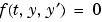 with consistent initial conditions, i.e.,
 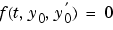 .
. ode15i provides an interface that is similar to that of the other MATLAB ODE solvers and is as easy to use. A supporting function decic helps you calculate consistent initial conditions. The existing functions odeset and odeget enable you to set integration properties that affect the problem solution. deval evaluates the numerical solution obtained with ode15i.
odextend, which is new in Version 7.0, enables you to extend the solution to an ODE created by an ODE solver.
bvp4c can now solve multipoint boundary value problems. To see an example of how to solve a three-point boundary value problem, enter threebvp. To see the code for the example, enter edit threebvp. Enter help bvp4c to learn more about bvp4c.
deval can now evaluate the derivative of the solution to an ODE as well as the solution itself. The command
New Output Function for Optimization Functions
In MATLAB 7.0, you can create an output function for several optimization functions in MATLAB. The optimization function calls the output function at each iteration of its algorithm. You can use the output function to obtain information about the data at each iteration or to stop the algorithm based on the current values of the data. You can use the output function with the following optimization functions:
See Calling an Output Function Iteratively for an example of how to use the output function.
New Support for Interpolation Functions
The following interpolation functions now have enhanced features:
interp1 -- The command YI = interp1(X,Y,XI) now accepts a multidimensional array Y and returns an array of the correct dimensions. If Y is an array of size [n,m1,m2,...,mk], interp1 performs interpolation for each m1-by-m2-by-...-mk value in Y. If XI is an array of size [d1,d2,...,dj], YI has size [d1,d2,...,dj,m1,m2,...,mk].
The command pp = interp1(X,Y,'method','pp') uses the specified method to generate the piecewise polynomial form (ppform) of Y. See the reference page for interp1 for information about the available methods.
interp2, interp3, and interpn -- You can now pass in a scalar argument, ExtrapVal, which these functions return for any values of XI and YI that lie outside the range of values spanned by X and Y defining the grid. For example,
returns the value of ExtrapVal for any values of XI or YI that are outside the range of values spanned by X and Y.
ppval now accepts multidimensional arrays returned by the spline function using the syntax
spline -- The command YY = spline(X,Y,XX) now accepts a multidimensional array Y and returns an array of the correct dimensions. Note that YY = spline(X,Y,XX) is the same as YY = ppval(spline(X,Y), XX).
If spline(X, Y) is scalar-valued, then YY is of the same size as XX. If spline(X, Y)is [D1,..,Dr]-valued, and XX has size [N1,...,Ns], then YY has size [D1,...,Dr, N1,...,Ns], where YY(:,...,:, J1,...,Js) is the value of spline(X, Y) at XX(J1,...,Js). There are two exceptions to this rule:
Enhanced sort Capabilities and Performance
Improved Performance
sort performance has been improved for numeric arrays of randomly ordered data. Although there is some performance improvement for all such numeric arrays, you should see the greatest improvement for integer arrays and multidimensional arrays.
Sort Direction
A new argument, mode, lets you specify whether sort returns the sorted array in ascending or descending order.
New Input Argument for Incomplete Gamma Function
The incomplete gamma function, gammainc, now accepts the input argument tail, using the syntax
tail specifies the tail of the incomplete gamma function when X is non-negative. The choices are for tail are 'lower' (the default) and 'upper'. The upper incomplete gamma function is defined as
New Function quadv Integrates Complex, Array-Valued Functions
The new function quadv integrates complex, array-valued functions.
New Form for Generalized Hessian
The function hess has a new syntax of the form
where A and B are square matrices, and returns an upper Hessenberg matrix AA, an upper triangular matrix BB, and unitary matrices Q and Z such that
New Output for polyeig
The function polyeig can now return a vector of condition numbers for the eigenvalues, when you call it with the syntax
At least one of A0 and Ap must be nonsingular. Large condition numbers imply that the problem is close to one with multiple eigenvalues.
New Trigonometric Functions For Angles in Degrees
The following new functions compute trigonometric functions of arguments in degrees.
| Function |
Purpose |
|---|---|
sind |
Compute the sine of an argument in degrees |
cosd |
Compute the cosine of an argument in degrees |
tand |
Compute the tangent of an argument in degrees |
cotd |
Compute the cotangent of an argument in degrees |
secd |
Compute the secant of an argument in degrees |
cscd |
Compute the cosecant of an argument in degrees |
The following new functions compute the inverse trigonometric functions are return the answer in degrees:
| Function |
Purpose |
|---|---|
asind |
Compute the inverse sine of an argument and return answer in degrees |
acosd |
Compute the inverse cosine of an argument and return answer in degrees |
atand |
Compute the inverse tangent of an argument and return answer in degrees |
acotd |
Compute the inverse cotangent of an argument and return answer in degrees |
asecd |
Compute the inverse secant of an argument and return answer in degrees |
acscd |
Compute the inverse cosecant of an argument and return answer in degrees |
New Functions for Computing Logarithms, Exponentials, and nth Roots
The following new functions compute logarithms, exponentials, and nth roots of real numbers.
| Function |
Purpose |
|---|---|
expm1 |
Compute exp(x)-1 accurately for small values of x |
log1p |
Compute log(1+x) accurately for small values of x |
nthroot |
Compute the real nth root of a real number |
Overriding the Default BLAS Library on Intel/Windows Systems
MATLAB uses the Basic Linear Algebra Subroutines (BLAS) libraries to speed up matrix multiplication and LAPACK-based functions like eig, svd, and \ (mldivide). At start-up, MATLAB selects the BLAS library to use.
For R14, MATLAB still uses the ATLAS BLAS libraries, however, on Windows systems running on Intel processors, you can switch the BLAS library that MATLAB uses to the Math Kernel Library (MKL) BLAS, provided by Intel.
If you want to take advantage of the potential performance enhancements provided by the Intel BLAS, you can set the value of the environment variable BLAS_VERSION to the name of the MKL library, mkl.dll. MATLAB uses the BLAS specified by this environment variable, if it exists.
To set the BLAS_VERSION environment variable, follow this procedure:
BLAS_VERSION and set the value of the variable to the name of the MKL library: mkl.dll.
Multithreading Disabled in Intel Math Kernel Library (MKL) BLAS
The Intel Math Kernel Library (MKL) is multithreaded in several areas. By default, this threading capability is disabled. To enable threading in the MKL library, set the value of the OMP_NUM_THREADS environment variable. Intel recommends setting the value of the OMP_NUM_THREADS variable to the number of processors you want to use in your application.
To set the value of this environment variable, follow the instructions outlined in Overriding the Default BLAS Library on Intel/Windows Systems.
Before enabling multithreading, read the Intel Math Kernel Library 6.1 for Windows Technical User Notes that explains certain limitations of this capability.
| | Publishing Results | Programming Features | |
© 1994-2005 The MathWorks, Inc.