xcorr (Signal Processing Toolbox)

Cross-correlation function

Syntax

c = xcorr(x,y)
c = xcorr(x)
c = xcorr(x,y,'option')
c = xcorr(x,'option')
c = xcorr(x,y,maxlags)
c = xcorr(x,maxlags)
c = xcorr(x,y,maxlags,'option')
c = xcorr(x,maxlags,'option')
[c,lags] = xcorr(...)

Description

xcorr estimates the cross-correlation sequence of a random process. Autocorrelation is handled as a special case.

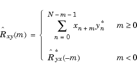
The true cross-correlation sequence is

where x_n and y_n are jointly stationary random processes, , and E {·} is the expected value operator. xcorr must estimate the sequence because, in practice, only a finite segment of one realization of the infinite-length random process is available.

c = xcorr(x,y) returns the cross-correlation sequence in a length 2*N-1 vector, where x and y are length N vectors (N>1). If x and y are not the same length, the shorter vector is zero-padded to the length of the longer vector.

By default, xcorr computes raw correlations with no normalization.

The output vector c has elements given by c(m) = R_xy(m-N), m=1, ..., 2N-1.

In general, the correlation function requires normalization to produce an accurate estimate (see below).

c = xcorr(x) is the autocorrelation sequence for the vector x. If x is an N-by-P matrix, c is a matrix with 2N-1 rows whose P² columns contain the cross-correlation sequences for all combinations of the columns of x. For more information on matrix processing with xcorr, see Multiple Channels.

c = xcorr(x,y,'option') specifies a normalization option for the cross-correlation, where 'option' is

'biased': Biased estimate of the cross-correlation function

'unbiased': Unbiased estimate of the cross-correlation function

'coeff': Normalizes the sequence so the autocorrelations at zero lag are identically 1.0.
'none', to use the raw, unscaled cross-correlations (default)

See reference [1] for more information on the properties of biased and unbiased correlation estimates.

c = xcorr(x,'option') specifies one of the above normalization options for the autocorrelation.

c = xcorr(x,y,maxlags) returns the cross-correlation sequence over the lag range [-maxlags:maxlags]. Output c has length 2*maxlags+1.

c = xcorr(x,maxlags) returns the autocorrelation sequence over the lag range [-maxlags:maxlags]. Output c has length 2*maxlags+1. If x is an N-by-P matrix, c is a matrix with 2*maxlags+1 rows whose P² columns contain the autocorrelation sequences for all combinations of the columns of x.

c = xcorr(x,y,maxlags,'option') specifies both a maximum number of lags and a scaling option for the cross-correlation.

c = xcorr(x,maxlags,'option') specifies both a maximum number of lags and a scaling option for the autocorrelation.

[c,lags] = xcorr(...) returns a vector of the lag indices at which c was estimated, with the range [-maxlags:maxlags]. When maxlags is not specified, the range of lags is [-N+1:N-1].

In all cases, the cross-correlation or autocorrelation computed by xcorr has the zeroth lag in the middle of the sequence, at element or row maxlags+1 (element or row N if maxlags is not specified).

Examples

The second output, lags, is useful for plotting the cross-correlation or autocorrelation. For example, the estimated autocorrelation of zero-mean Gaussian white noise c_ww(m) can be displayed for -10 m 10 using:

ww = randn(1000,1);
[c_ww,lags] = xcorr(ww,10,'coeff');
stem(lags,c_ww)

Swapping the x and y input arguments reverses (and conjugates) the output correlation sequence. For row vectors, the resulting sequences are reversed left to right; for column vectors, up and down. The following example illustrates this property (mat2str is used for a compact display of complex numbers):

x = [1,2i,3]; y = [4,5,6];
[c1,lags] = xcorr(x,y);
c1 = mat2str(c1,2), lags
c1 =
    [6-i*8.9e-016 5+i*12 22+i*10 15+i*8 12+i*8.9e-016]
lags =
    -2    -1     0     1     2
c2 = conj(fliplr(xcorr(y,x)));
c2 = mat2str(c2,2)
c2 =
    [6-i*8.9e-016 5+i*12 22+i*10 15+i*8 12+i*8.9e-016]

For the case where input argument x is a matrix, the output columns are arranged so that extracting a row and rearranging it into a square array produces the cross-correlation matrix corresponding to the lag of the chosen row. For example, the cross-correlation at zero lag can be retrieved by:

randn('state',0)
X = randn(2,2);
[M,P] = size(X);
c = xcorr(X);
c0 = zeros(P); c0(:) = c(M,:)   % Extract zero-lag row
c0 =
    2.9613   -0.5334
   -0.5334    0.0985

You can calculate the matrix of correlation coefficients that the MATLAB function corrcoef generates by substituting:

```
c = xcov(X,'coef')
```

in the last example. The function xcov subtracts the mean and then calls xcorr.

Use fftshift to move the second half of the sequence starting at the zeroth lag to the front of the sequence. fftshift swaps the first and second halves of a sequence.

Algorithm

For more information on estimating covariance and correlation functions, see [1].

See Also

conv, corrcoef, cov, xcorr2, xcov

References

[1] Orfanidis, S.J., Optimum Signal Processing. An Introduction. 2nd Edition, Prentice-Hall, Englewood Cliffs, NJ, 1996.

wvtool xcorr2