MATLAB Function Reference

coneplot

Plot velocity vectors as cones in a 3-D vector field

Syntax

• coneplot(X,Y,Z,U,V,W,Cx,Cy,Cz)
  coneplot(U,V,W,Cx,Cy,Cz)
  coneplot(...,s)
  coneplot(...,color)
  coneplot(...,'quiver')
  coneplot(...,'method')
  coneplot(X,Y,Z,U,V,W,'nointerp')
  comeplot(axes_handle,...)
  h = coneplot(...)
  

Description

coneplot(X,Y,Z,U,V,W,Cx,Cy,Cz) plots velocity vectors as cones pointing in the direction of the velocity vector and having a length proportional to the magnitude of the velocity vector.

• X, Y, Z define the coordinates for the vector field.
• U, V, W define the vector field. These arrays must be the same size, monotonic, and 3-D plaid (such as the data produced by meshgrid).
• Cx, Cy, Cz define the location of the cones in the vector field. The section Starting Points for Stream Plots in Visualization Techniques provides more information on defining starting points.

coneplot(U,V,W,Cx,Cy,Cz) (omitting the X, Y, and Z arguments) assumes [X,Y,Z] = meshgrid(1:n,1:m,1:p) where [m,n,p]= size(U).

coneplot(...,s) MATLAB automatically scales the cones to fit the graph and then stretches them by the scale factor s. If you do not specify a value for s, MATLAB uses a value of 1. Use s = 0 to plot the cones without automatic scaling.

coneplot(...,color) interpolates the array color onto the vector field and then colors the cones according to the interpolated values. The size of the color array must be the same size as the U, V, W arrays. This option works only with cones (i.e., not with the quiver option).

coneplot(...,'quiver') draws arrows instead of cones (see quiver3 for an illustration of a quiver plot).

coneplot(...,'method') specifies the interpolation method to use. method can be linear, cubic, or nearest. linear is the default (see interp3 for a discussion of these interpolation methods).

coneplot(X,Y,Z,U,V,W,'nointerp') does not interpolate the positions of the cones into the volume. The cones are drawn at positions defined by X, Y, Z and are oriented according to U, V, W. Arrays X, Y, Z, U, V, W must all be the same size.

coneplot(axes_handle,...) plots into the axes with handle axes_handle instead of the current axes (gca).

h = coneplot(...) returns the handle to the patch object used to draw the cones. You can use the set command to change the properties of the cones.

Remarks

coneplot automatically scales the cones to fit the graph, while keeping them in proportion to the respective velocity vectors.

It is usually best to set the data aspect ratio of the axes before calling coneplot. You can set the ratio using the daspect command,

• daspect([1,1,1])
  

Examples

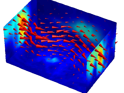
This example plots the velocity vector cones for vector volume data representing the motion of air through a rectangular region of space. The final graph employs a number of enhancements to visualize the data more effectively. These include

• Cone plots indicate the magnitude and direction of the wind velocity.
• Slice planes placed at the limits of the data range provide a visual context for the cone plots within the volume.
• Directional lighting provides visual cues to the orientation of the cones.
• View adjustments compose the scene to best reveal the information content of the data by selecting the view point, projection type, and magnification.

1. Load and Inspect Data

The winds data set contains six 3-D arrays: u, v, and w specify the vector components at each of the coordinates specified in x, y, and z. The coordinates define a lattice grid structure where the data is sampled within the volume.

It is useful to establish the range of the data to place the slice planes and to specify where you want the cone plots (min, max).

• load wind
  xmin = min(x(:));
  xmax = max(x(:));
  ymin = min(y(:));
  ymax = max(y(:));
  zmin = min(z(:));
  

2. Create the Cone Plot

• Decide where in data space you want to plot cones. This example selects the full range of x and y in eight steps and the range 3 to 15 in four steps in z (linspace, meshgrid).
• Use daspect to set the data aspect ratio of the axes before calling coneplot so MATLAB can determine the proper size of the cones.
• Draw the cones, setting the scale factor to 5 to make the cones larger than the default size.
• Set the coloring of each cone (FaceColor, EdgeColor).

• daspect([2,2,1])
  xrange = linspace(xmin,xmax,8);
  yrange = linspace(ymin,ymax,8);
  zrange = 3:4:15;
  [cx cy cz] = meshgrid(xrange,yrange,zrange);
  hcones = coneplot(x,y,z,u,v,w,cx,cy,cz,5);
  set(hcones,'FaceColor','red','EdgeColor','none')
  

3. Add the Slice Planes

• Calculate the magnitude of the vector field (which represents wind speed) to generate scalar data for the slice command.
• Create slice planes along the x-axis at xmin and xmax, along the y-axis at ymax, and along the z-axis at zmin.
• Specify interpolated face color so the slice coloring indicates wind speed and do not draw edges (hold, slice, FaceColor, EdgeColor).

• hold on
  wind_speed = sqrt(u.^2 + v.^2 + w.^2);
  hsurfaces = slice(x,y,z,wind_speed,[xmin,xmax],ymax,zmin);
  set(hsurfaces,'FaceColor','interp','EdgeColor','none')
  hold off
  

4. Define the View

• Use the axis command to set the axis limits equal to the range of the data.
• Orient the view to azimuth = 30 and elevation = 40 (rotate3d is a useful command for selecting the best view).
• Select perspective projection to provide a more realistic looking volume (camproj).
• Zoom in on the scene a little to make the plot as large as possible (camzoom).

• axis tight; view(30,40); axis off
  camproj perspective; camzoom(1.5)
  

5. Add Lighting to the Scene

The light source affects both the slice planes (surfaces) and the cone plots (patches). However, you can set the lighting characteristics of each independently.

• Add a light source to the right of the camera and use Phong lighting to give the cones and slice planes a smooth, three-dimensional appearance (camlight, lighting).
• Increase the value of the AmbientStrength property for each slice plane to improve the visibility of the dark blue colors. (Note that you can also specify a different colormap to change the coloring of the slice planes.)
• Increase the value of the DiffuseStrength property of the cones to brighten particularly those cones not showing specular reflections.

• camlight right; lighting phong
  set(hsurfaces,'AmbientStrength',.6)
  set(hcones,'DiffuseStrength',.8)
  
  
  

See Also

isosurface, patch, reducevolume, smooth3, streamline, stream2, stream3, subvolume

Volume Visualization for related functions

condest

conj

© 1994-2005 The MathWorks, Inc.