3-D Visualization

Visualizing MRI Data

An example of scalar data includes Magnetic Resonance Imaging (MRI) data. This data typically contains a number of slice planes taken through a volume, such as the human body. MATLAB includes an MRI data set that contains 27 image slices of a human head. This section describes some useful techniques for visualizing MRI data.

Example -- Ways to Display MRI Data

This example illustrate the following techniques applied to MRI data:

• A series of 2-D images representing slices through the head
• 2-D and 3-D contour slices taken at arbitrary locations within the data
• An isosurface with isocaps showing a cross section of the interior

Changing the Data Format

The MRI data, D, is stored as a 128-by-128-by-1-by-27 array. The third array dimension is used typically for the image color data. However, since these are indexed images (a colormap, map, is also loaded) there is no information in the third dimension, which you can remove using the squeeze command. The result is a 128-by-128-by-27 array.

The first step is to load the data and transform the data array from 4-D to 3-D.

• load mri
  D = squeeze(D);
  

Displaying Images of MRI Data

To display one of the MRI images, use the image command, indexing into the data array to obtain the eighth image. Then adjust axis scaling, and install the MRI colormap, which was loaded along with the data.

• image_num = 8;
  image(D(:,:,image_num))
  axis image
  colormap(map)
  
  
  

Save the x- and y-axis limits for use in the next part of the example.

• x = xlim;
  y = ylim;
  

Displaying a 2-D Contour Slice

You can treat this MRI data as a volume because it is a collection of slices taken progressively through the 3-D object. Use contourslice to display a contour plot of a slice of the volume. To create a contour plot with the same orientation and size as the image created in the first part of this example, adjust the y-axis direction (axis), set the limits (xlim, ylim), and set the data aspect ratio (daspect).

• contourslice(D,[],[],image_num)
  axis ij
  xlim(x)
  ylim(y)
  daspect([1,1,1])
  colormap('default')
  

This contour plot uses the figure colormap to map color to contour value.

Displaying 3-D Contour Slices

Unlike images, which are 2-D objects, contour slices are 3-D objects that you can display in any orientation. For example, you can display four contour slices in a 3-D view. To improve the visibility of the contour line, increase the LineWidth to 2 points (one point equals 1/72 of an inch).

• phandles = contourslice(D,[],[],[1,12,19,27],8);
  view(3); axis tight
  set(phandles,'LineWidth',2)
  
  
  

Displaying an Isosurface

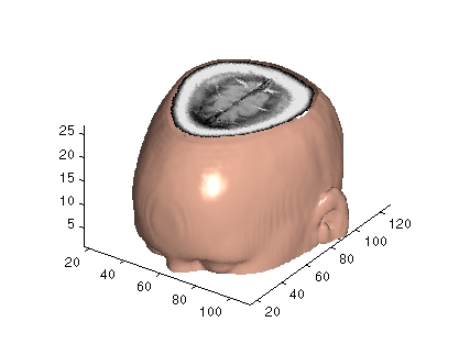
You can use isosurfaces to display the overall structure of a volume. When combined with isocaps, this technique can reveal information about data on the interior of the isosurface.

First, smooth the data with smooth3; then use isosurface to calculate the isodata. Use patch to display this data as a graphics object.

• Ds = smooth3(D);
  hiso = patch(isosurface(Ds,5),...
      'FaceColor',[1,.75,.65],...
      'EdgeColor','none');
  

Adding an Isocap to Show a Cutaway Surface

Use isocaps to calculate the data for another patch that is displayed at the same isovalue (5) as the surface. Use the unsmoothed data (D) to show details of the interior. You can see this as the sliced-away top of the head.

• hcap = patch(isocaps(D,5),...
      'FaceColor','interp',...
      'EdgeColor','none');
  colormap(map)
  

Defining the View

Define the view and set the aspect ratio (view, axis, daspect).

• view(45,30) 
  axis tight 
  daspect([1,1,.4])
  

Add Lighting

Add lighting and recalculate the surface normals based on the gradient of the volume data, which produces smoother lighting (camlight, lighting, isonormals). Increase the AmbientStrength property of the isocap to brighten the coloring without affecting the isosurface. Set the SpecularColorReflectance of the isosurface to make the color of the specular reflected light closer to the color of the isosurface; then set the SpecularExponent to reduce the size of the specular spot.

• lightangle(45,30); 
  set(gcf,'Renderer','zbuffer'); lighting phong
  isonormals(Ds,hiso)
  set(hcap,'AmbientStrength',.6)
  set(hiso,'SpecularColorReflectance',0,'SpecularExponent',50)
  
  
  

The isocap uses interpolated face coloring, which means the figure colormap determines the coloring of the patch. This example uses the colormap supplied with the data.

To display isocaps at other data values, try changing the isosurface value or use the subvolume command. See the isocaps and subvolume reference pages for examples.

Visualizing Scalar Volume Data

Exploring Volumes with Slice Planes

© 1994-2005 The MathWorks, Inc.