

| Wavelet Toolbox |   |
Continuous Analysis Using the Graphical Interface
We now use the Continuous Wavelet 1-D tool to analyze the same noisy sinusoidal signal we examined earlier using the command line interface in Continuous Analysis Using the Command Line.
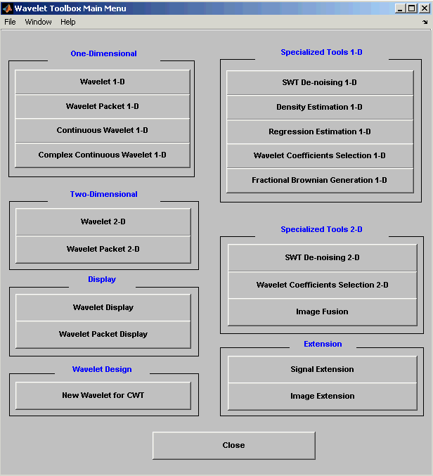
Click the Continuous Wavelet 1-D menu item.
The continuous wavelet analysis tool for one-dimensional signal data appears.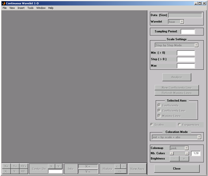
 Load Signal menu option.
When the Load Signal dialog box appears, select the demo MAT-file noissin.mat, which should reside in the MATLAB directory toolbox/wavelet/wavedemo. Click the OK button.
The noisy sinusoidal signal is loaded into the Continuous Wavelet 1-D tool.
The default value for the sampling period is equal to 1 (second).
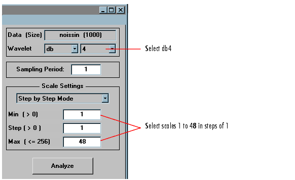
db4 wavelet at scales 1 through 48, just as we did using command line functions in the previous section.
In the upper right portion of the Continuous Wavelet 1-D tool, select the db4 wavelet and scales 1-48.
After a pause for computation, the tool displays the coefficients plot, the coefficients line plot corresponding to the scale a = 24, and the local maxima plot, which displays the chaining across scales (from a = 48 down to a = 1) of the coefficients local maxima.
9 below to know, more precisely, how to select the desired scale.
Click the New Coefficients Line button. The tool updates the plot.

Hold down the right mouse button over the coefficients plot, the position of the mouse is given by the Info frame (located at the bottom of the screen) in terms of location (X) and scale (Sca).
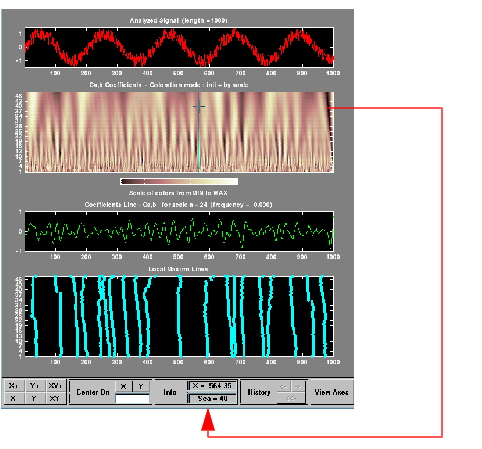
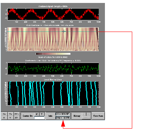
This facility allows you to interpret scale in terms of an associated pseudo-frequency, which depends on the wavelet and the sampling period. For more information on the connection between scale and frequency, see "How to Connect Scale to Frequency?.
Deselect the last two plots using the check boxes in the Selected Axes frame
Click the X+ button (located at the bottom of the screen) to zoom horizontally only.

The Continuous Wavelet 1-D tool enlarges the displayed signal and coefficients plot (for more information on zooming, see Connection of Plots).
As with the command line analysis on the preceding pages, you can change the scales or the analyzing wavelet and repeat the analysis. To do this, just edit the necessary fields and press the Analyze button.
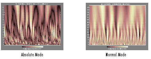
More generally, the coefficients coloration can be done in several different ways. For more details on the Coloration Mode, see Controlling the Coloration Mode.
Choose either one of the absolute modes or normal modes from the Coloration Mode menu. In normal modes, the colors are scaled between the minimum and maximum of the coefficients. In absolute modes, the colors are scaled between zero and the maximum absolute value of the coefficients.
The coefficients plot is redisplayed in the mode you select.
 | Continuous Analysis Using the Command Line | Importing and Exporting Information from the Graphical Interface |  |
© 1994-2005 The MathWorks, Inc.