dwt (Wavelet Toolbox)

Single-level discrete 1-D wavelet transform

Syntax

[cA,cD] = dwt(X,'wname')
[cA,cD] = dwt(X,'wname','mode',MODE)
[cA,cD] = dwt(X,Lo_D,Hi_D)
[cA,cD] = dwt(X,Lo_D,Hi_D,'mode',MODE)

Description

The dwt command performs a single-level one-dimensional wavelet decomposition with respect to either a particular wavelet ('wname', see wfilters for more information) or particular wavelet decomposition filters (Lo_D and Hi_D) that you specify.

[cA,cD] = dwt(X,'wname') computes the approximation coefficients vector cA and detail coefficients vector cD, obtained by a wavelet decomposition of the vector X. The string 'wname' contains the wavelet name.

[cA,cD] = dwt(X,Lo_D,Hi_D) computes the wavelet decomposition as above, given these filters as input:

Lo_D is the decomposition low-pass filter.
Hi_D is the decomposition high-pass filter.

Lo_D and Hi_D must be the same length.

Let lx = the length of X and lf = the length of the filters Lo_D and Hi_D; then length(cA) = length(cD) = la where la = ceil(lx/2), if the DWT extension mode is set to periodization. For the other extension modes, la = floor(lx+lf-1)/2).

For more information about the different Discrete Wavelet Transform extension modes, see dwtmode.

[cA,cD] = dwt(...,'mode',MODE) computes the wavelet decomposition with the extension mode MODE that you specify. MODE is a string containing the desired extension mode.

Example:

```
[cA,cD] = dwt(x,'db1','mode','sym');
```

Examples

% The current extension mode is zero-padding (see dwtmode).

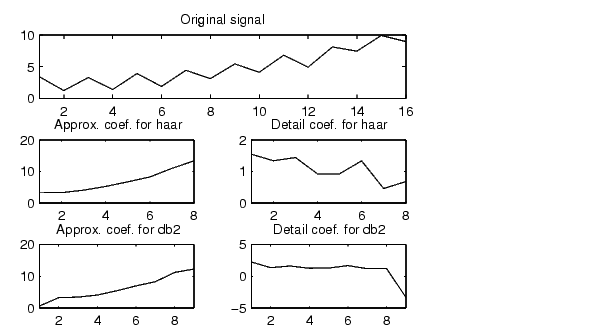
% Construct elementary original one-dimensional signal. 
randn('seed',531316785) 
s = 2 + kron(ones(1,8),[1 -1]) + ...
    ((1:16).^2)/32 + 0.2*randn(1,16);

% Perform single-level discrete wavelet transform of s by haar.
[ca1,cd1] = dwt(s,'haar'); 
subplot(311); plot(s); title('Original signal'); 
subplot(323); plot(ca1); title('Approx. coef. for haar'); 
subplot(324); plot(cd1); title('Detail coef. for haar');

% For a given wavelet, compute the two associated decomposition 
% filters and compute approximation and detail coefficients 
% using directly the filters. 
[Lo_D,Hi_D] = wfilters('haar','d'); 
[ca1,cd1] = dwt(s,Lo_D,Hi_D);

% Perform single-level discrete wavelet transform of s by db2
% and observe edge effects for last coefficients.
% These extra coefficients are only used to ensure exact 
% global reconstruction.
[ca2,cd2] = dwt(s,'db2');
subplot(325); plot(ca2); title('Approx. coef. for db2'); 
subplot(326); plot(cd2); title('Detail coef. for db2');

% Editing some graphical properties,
% the following figure is generated.

Algorithm

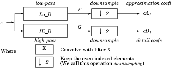
Starting from a signal s, two sets of coefficients are computed: approximation coefficients CA₁, and detail coefficients CD₁. These vectors are obtained by convolving s with the low-pass filter Lo_D for approximation and with the high-pass filter Hi_D for detail, followed by dyadic decimation.

More precisely, the first step is

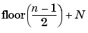
The length of each filter is equal to 2N. If n = length(s), the signals F and G are of length n + 2N - 1, and then the coefficients CA₁ and CD₁ are of length

To deal with signal-end effects involved by a convolution-based algorithm, a global variable managed by dwtmode is used. This variable defines the kind of signal extension mode used. The possible options include zero-padding (used in the previous example) and symmetric extension, which is the default mode.

See Also

dwtmode, idwt, wavedec, waveinfo

References

Daubechies, I. (1992), Ten lectures on wavelets, CBMS-NSF conference series in applied mathematics. SIAM Ed.

Mallat, S. (1989), "A theory for multiresolution signal decomposition: the wavelet representation," IEEE Pattern Anal. and Machine Intell., vol. 11,
no. 7, pp. 674-693.

Meyer, Y. (1990), Ondelettes et opérateurs, Tome 1, Hermann Ed. (English translation: Wavelets and operators, Cambridge Univ. Press. 1993.)

dtree dwt2