| Wavelet Toolbox | |
Syntax
Description
F = scal2frq(A,'wname',DELTA) returns the pseudo-frequencies corresponding to the scales given by A, the wavelet function 'wname' (see wavefun for more information) and the sampling period DELTA.
scal2frq(A,'wname') is equivalent to scal2frq(A,'wname',1).
One of the most frequently asked question is, "How does one map a scale, for a given wavelet and a sampling period, to a kind of frequency?".
The answer can only be given in a broad sense and it's better to speak about the pseudo-frequency corresponding to a scale.
A way to do it is to compute the center frequency, Fc, of the wavelet and to use the following relationship.

Fc is the center frequency of a wavelet in Hz.
Fa is the pseudo-frequency corresponding to the scale a, in Hz.
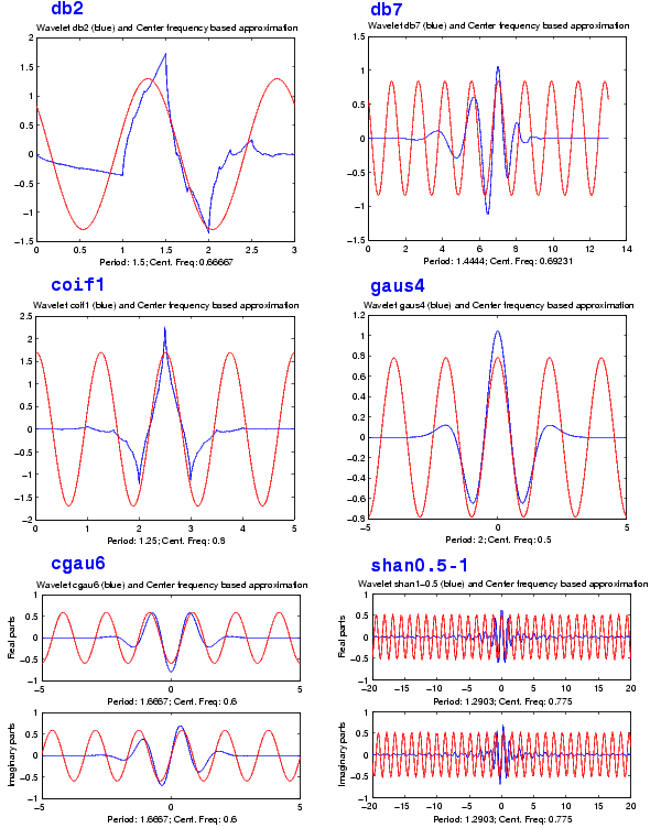
The idea is to associate with a given wavelet a purely periodic signal of frequency Fc. The frequency maximizing the fft of the wavelet modulus is Fc. The function centfrq can be used to compute the center frequency and it allows the plotting of the wavelet with the associated approximation based on the center frequency. The figure on the next page shows some examples generated using the centfrq function.
Center Frequencies for Real and Complex Wavelets
As you can see, the center frequency based approximation captures the main wavelet oscillations. So the center frequency is a convenient and simple characterization of the leading dominant frequency of the wavelet.
If we accept to associate the frequency Fc to the wavelet function then, when the wavelet is dilated by a factor a, this center frequency becomes Fc / a. Lastly, if the underlying sampling period is  , it is natural to associate to the scale a the frequency:

The function scal2frq computes this correspondence.
To illustrate the behavior of this procedure, let us consider the following simple test. We generate sine functions of sensible frequencies F0. For each function, we shall try to detect this frequency by a wavelet decomposition followed by a translation of scale to frequency. More precisely, after a discrete wavelet decomposition, we identify the scale a* corresponding to the maximum value of the energy of the coefficients. The translated frequency F* is then given by
The F* values are close to the chosen F0. The plots at the end of example 2, presents the periods instead of frequencies. If we change slightly the F0 values, the results remain satisfactory.
Examples
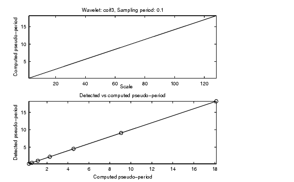
% Set sampling period and wavelet name.
delta = 0.1; wname = 'coif3';

% Define scales.
amax = 7; a = 2.^[1:amax];

% Compute associated pseudo-frequencies.
f = scal2frq(a,wname,delta);

% Compute associated pseudo-periods.
per = 1./f;


% Display information.
disp('    Scale    Frequency  Period')
disp([a' f' per'])

    Scale    Frequency  Period

    2.0000    3.5294    0.2833
    4.0000    1.7647    0.5667
    8.0000    0.8824    1.1333
   16.0000    0.4412    2.2667
   32.0000    0.2206    4.5333
   64.0000    0.1103    9.0667
  128.0000    0.0551   18.1333
% Set sampling period and wavelet name.
delta = 0.1; wname = 'coif3';

% Define scales.
amax = 7;
a = 2.^[1:amax];

% Compute associated pseudo-frequencies.
f = scal2frq(a,wname,delta);

% Compute associated pseudo-periods.
per = 1./f;

% Plot pseudo-periods versus scales.
subplot(211), plot(a,per)
title(['Wavelet: ',wname, ', Sampling period: ',num2str(delta)])
xlabel('Scale')
ylabel('Computed pseudo-period')

% For each scale 2^i:
% - generate a sine function of period per(i);
% - perform a wavelet decomposition;
% - identify the highest energy level;
% - compute the detected pseudo-period.

for i = 1:amax
   % Generate sine function of period
   % per(i) at sampling period delta.
   t = 0:delta:100;
   x = sin((t.*2*pi)/per(i));
   % Decompose x at level 9.
   [c,l] = wavedec(x,9,wname);

   % Estimate standard deviation of detail coefficients.
   stdc = wnoisest(c,l,[1:amax]);
   % Compute identified period.
   [y,jmax] = max(stdc);
   idper(i) = per(jmax);
end

% Compare the detected and computed pseudo-periods.
subplot(212), plot(per,idper,'o',per,per)
title('Detected vs computed pseudo-period')
xlabel('Computed pseudo-period')
ylabel('Detected pseudo-period')
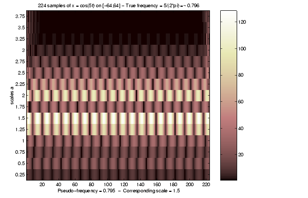
This example demonstrates that, starting from the periodic function x(t) = cos(5t), the scal2frq function translates the scale corresponding to the maximum value of the CWT coefficients to a pseudo-frequency (0.795), which is near to the true frequency (5/(2*pi) =~ 0.796).
% Set wavelet name, interval and number of samples.wname = 'db10';A = -64; B = 64; P = 224;% Compute the sampling period and the sampled function, % and the true frequency. delta = (B-A)/(P-1); t = linspace(A,B,P); omega = 5; x = cos(omega*t); freq = omega/(2*pi); % Set scales and use scal2frq to compute the array % of pseudo-frequencies. scales = [0.25:0.25:3.75]; TAB_PF = scal2frq(scales,wname,delta); % Compute the nearest pseudo-frequency % and the corresponding scale. [dummy,ind] = min(abs(TAB_PF-freq)); freq_APP = TAB_PF(ind); scale_APP = scales(ind); % Continuous analysis and plot.str1 = ['224 samples of x = cos(5t) on [-64,64] - ' ...'True frequency = 5/(2*pi) =~ ' num2str(freq,3)];str2 = ['Array of pseudo-frequencies and scales: '];str3 = [num2str([TAB_PF',scales'],3)];str4 = ['Pseudo-frequency = ' num2str(freq_APP,3)];str5 = ['Corresponding scale = ' num2str(scale_APP,3)];figure; cwt(x,scales,wname,'plot'); ax = gca; colorbaraxTITL = get(ax,'title');axXLAB = get(ax,'xlabel');set(axTITL,'String',str1)set(axXLAB,'String',[str4,' - ' str5])clc ; disp(strvcat(' ',str1,' ',str2,str3,' ',str4,str5))224 samples of x = cos(5t) on [-64,64] - True frequency = 5/(2*pi) =~0.796 Array of pseudo-frequencies and scales: 4.77 0.25 2.38 0.5 1.59 0.75 1.19 1 0.954 1.25 0.795 1.5 0.681 1.75 0.596 2 . . . . 0.341 3.5 0.318 3.75 Pseudo-frequency = 0.795 Corresponding scale = 1.5
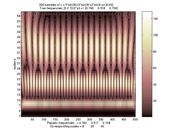
This example demonstrates that, starting from the periodic function x(t) = 5*sin(5t)+3*sin(2t)+2*sin(t), the scal2frq function translates the scales corresponding to the maximum values of the CWT coefficients to pseudo-frequencies ([0.796 0.318 0.159]), which are near to the true frequencies ([5 2 1] / (2*pi) =~ [0.796 0.318 0.159]).
% Set wavelet name,interval and number of samples.wname = 'morl';A = 0; B = 64; P = 500;% Compute the sampling period and the sampled function,% and the true frequencies.t = linspace(A,B,P);delta = (B-A)/(P-1);tab_OMEGA = [5,2,1];tab_FREQ = tab_OMEGA/(2*pi);tab_COEFS = [5,3,2];x = zeros(1,P);for k = 1:3;x = x+tab_COEFS(k)*sin(tab_OMEGA(k)*t);end% Set scales and use scal2frq to compute the array% of pseudo-frequencies.scales = [1:1:60];tab_PF = scal2frq(scales,wname,delta);% Compute the nearest pseudo-frequencies% and the corresponding scales.for k=1:3[dummy,ind] = min(abs(tab_PF-tab_FREQ(k)));PF_app(k) = tab_PF(ind);SC_app(k) = scales(ind);end% Continuous analysis and plot.str1 = strvcat( ...'500 samples of x = 5*sin(5t)+3*sin(2t)+2*sin(t) on [0,64]',...['True frequencies (in Hz): [5 2 1]/(2*pi) =~ [' ...num2str(tab_FREQ,3) ']' ] ...);str2 = ['Array of pseudo-frequencies and scales: '];str3 = [num2str([tab_PF',scales'],3)];str4 = ['Pseudo-frequencies = ' num2str(PF_app,3)];str5 = ['Corresponding scales = ' num2str(SC_app,3)];figure; cwt(x,scales,wname,'plot'); ax = gca; colorbaraxTITL = get(ax,'title');axXLAB = get(ax,'xlabel');set(axTITL,'String',str1)set(axXLAB,'String',strvcat(str4, str5))clc; disp(strvcat(' ',str1,' ',str2,str3,' ',str4,str5))500 samples of x = 5*sin(5t)+3*sin(2t)+2*sin(t) on [0,64] True frequencies(in Hz): [5 2 1]/(2*pi) =~[0.796 0.318 0.159] Array of pseudo-frequencies and scales: 6.33 1 3.17 2 2.11 3 1.58 4 1.27 5 1.06 6 0.905 7 0.792 8 0.704 9 0.633 10 . . . . . . . . 0.122 52 0.12 53 0.117 54 0.115 55 0.113 56 0.111 57 0.109 58 0.107 59 0.106 60 Pseudo-frequencies = 0.792 0.317 0.158 Corresponding scales = 8 20 40
See Also
centfrq
References
Abry, P. (1997), Ondelettes et turbulence. Multirésolutions, algorithmes de décomposition, invariance d'échelles, Diderot Editeur, Paris.
| | readtree | set | |
© 1994-2005 The MathWorks, Inc.
 is the sampling period.