interp1 (MATLAB Functions)

One-dimensional data interpolation (table lookup)

Syntax

yi = interp1(x,Y,xi)
yi = interp1(Y,xi)
yi = interp1(x,Y,xi,method)
yi = interp1(x,Y,xi,method,'extrap')
yi = interp1(x,Y,xi,method,extrapval)
pp = interp1(x,Y,method,'pp')

Description

yi = interp1(x,Y,xi) interpolates to find yi, the values of the underlying function Y at the points in the vector or array xi. x must be a vector. Y can be a scalar, a vector, or an array of any dimension, subject to the following conditions:

If Y is a scalar or vector, it must have the same length as x. A scalar value for x or Y is expanded to have the same length as the other. xi can be a scalar, a vector, or a multidimensional array, and yi has the same size as xi.
If Y is an array that is not a vector, the size of Y must have the form [n,d1,d2,...,dk], where n is the length of x. The interpolation is performed for each d1-by-d2-by-...-dk value in Y. The sizes of xi and yi are related as follows:

If xi is a scalar or vector, size(yi) equals [length(xi), d1, d2, ..., dk].
If xi is an array of size [m1,m2,...,mj], yi has size [m1,m2,...,mj,d1,d2,...,dk].

yi = interp1(Y,xi) assumes that x = 1:N, where N is the length of Y for vector Y, or size(Y,1) for matrix Y.

yi = interp1(x,Y,xi,method) interpolates using alternative methods:

'nearest'
Nearest neighbor interpolation

'linear'
Linear interpolation (default)

'spline'
Cubic spline interpolation

'pchip'
Piecewise cubic Hermite interpolation

'cubic'
(Same as 'pchip')

'v5cubic'
Cubic interpolation used in MATLAB 5

`'nearest'`	Nearest neighbor interpolation
`'linear'`	Linear interpolation (default)
`'spline'`	Cubic spline interpolation
`'pchip'`	Piecewise cubic Hermite interpolation
`'cubic'`	(Same as '`pchip'`)
`'v5cubic'`	Cubic interpolation used in MATLAB 5

For the 'nearest', 'linear', and 'v5cubic' methods, interp1(x,Y,xi,method) returns NaN for any element of xi that is outside the interval spanned by x. For all other methods, interp1 performs extrapolation for out of range values.

yi = interp1(x,Y,xi,method,'extrap') uses the specified method to perform extrapolation for out of range values.

yi = interp1(x,Y,xi,method,extrapval) returns the scalar extrapval for out of range values. NaN and 0 are often used for extrapval.

pp = interp1(x,Y,method,'pp') uses the specified method to generate the piecewise polynomial form (ppform) of Y. You can use any of the methods in the preceding table, except for 'v5cubic'.

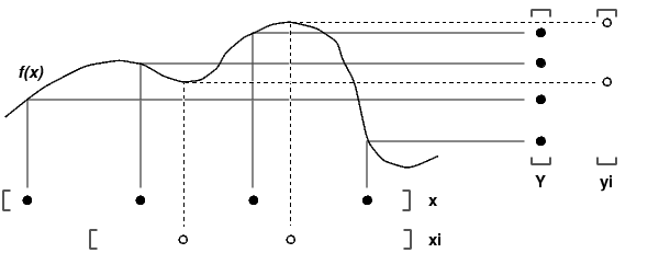
The interp1 command interpolates between data points. It finds values at intermediate points, of a one-dimensional function that underlies the data. This function is shown below, along with the relationship between vectors x, Y, xi, and yi.

Interpolation is the same operation as table lookup. Described in table lookup terms, the table is [x,Y] and interp1 looks up the elements of xi in x, and, based upon their locations, returns values yi interpolated within the elements of Y.

Note interp1q is quicker than interp1 on non-uniformly spaced data because it does no input checking. For interp1q to work properly, x must be a monotonically increasing column vector and Y must be a column vector or matrix with length(X) rows. Type help interp1q at the command line for more information.

Examples

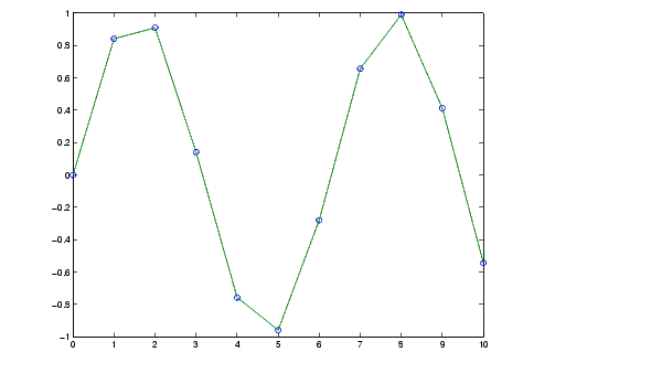
Example 1. Generate a coarse sine curve and interpolate over a finer abscissa.

x = 0:10; 
y = sin(x); 
xi = 0:.25:10; 
yi = interp1(x,y,xi); 
plot(x,y,'o',xi,yi)

Example 2. The following multidimensional example creates 2-by-2 matrices of interpolated function values, one matrix for each of the three functions x², x³, and x⁴.

x = [1:10]'; y = [ x.^2, x.^3, x.^4 ]; 
xi = [1.5, 1.75; 7.5, 7.75]; 
yi = interp1(x,y,xi);

The result yi has size 2-by-2-by-3.

```
size(yi)

ans =

     2     2     3
```

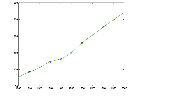
Example 3. Here are two vectors representing the census years from 1900 to 1990 and the corresponding United States population in millions of people.

t = 1900:10:1990;
p = [75.995  91.972  105.711  123.203  131.669...
     150.697  179.323  203.212  226.505  249.633];

The expression interp1(t,p,1975) interpolates within the census data to estimate the population in 1975. The result is

```
ans =
    214.8585
```

Now interpolate within the data at every year from 1900 to 2000, and plot the result.

 x = 1900:1:2000;
 y = interp1(t,p,x,'spline');
 plot(t,p,'o',x,y)

Sometimes it is more convenient to think of interpolation in table lookup terms, where the data are stored in a single table. If a portion of the census data is stored in a single 5-by-2 table,

tab =
    1950    150.697
    1960    179.323
    1970    203.212
    1980    226.505
    1990    249.633

then the population in 1975, obtained by table lookup within the matrix tab, is

p = interp1(tab(:,1),tab(:,2),1975)
p =
    214.8585

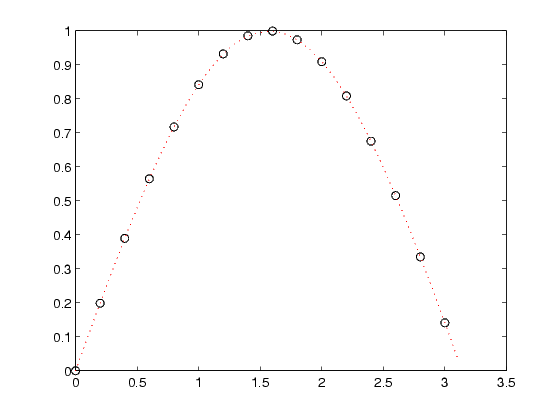
Example 4. The following example uses the 'cubic' method to generate the piecewise polynomial form (ppform) of Y, and then evaluates the result using ppval.

x = 0:.2:pi; y = sin(x);
pp = interp1(x,y,'cubic','pp');
xi = 0:.1:pi;
yi = ppval(pp,xi);
plot(x,y,'ko'), hold on, plot(xi,yi,'r:'), hold off

Algorithm

The interp1 command is a MATLAB M-file. The 'nearest' and 'linear' methods have straightforward implementations.

For the 'spline' method, interp1 calls a function spline that uses the functions ppval, mkpp, and unmkpp. These routines form a small suite of functions for working with piecewise polynomials. spline uses them to perform the cubic spline interpolation. For access to more advanced features, see the spline reference page, the M-file help for these functions, and the Spline Toolbox.

For the 'pchip' and 'cubic' methods, interp1 calls a function pchip that performs piecewise cubic interpolation within the vectors x and y. This method preserves monotonicity and the shape of the data. See the pchip reference page for more information.

See Also

interpft, interp2, interp3, interpn, pchip, spline

References

[1] de Boor, C., A Practical Guide to Splines, Springer-Verlag, 1978.

int8, int16, int32, int64 interp2